Deep-dive — sphere, cylinder, pinhole: one camera, three images, and the pixel math that links them¶

Run alongside this: python examples/08_reproject_sphere_cylinder.py (after the setup). It writes the three images below and prints the round-trip residual that proves the maps are exact inverses.

You may have seen a fisheye frame "unwrapped" onto a cylinder or a sphere, with landmarks drawn on the curved surface, and wondered: is that real geometry, or just a pretty picture?

Can a non-flat image even have intrinsics you can do 2D/3D work with?

Short answer: it's real, and the sphere version is more fundamental than the flat image you started with.

This deep-dive shows why, gives you the exact pixel↔pixel formulas to move between sphere ↔ cylinder ↔ pinhole, and proves they round-trip to ~1e-13 px on the bundled real fisheye.

You'll learn - Why a central camera is fully described by a bijection between unit-sphere rays and pixels, and how sphere, cylinder, and pinhole are three different "chart" formulas for that same bijection. - The exact pixel↔pixel conversion formulas between sphere, cylinder, and pinhole charts, verified to round-trip to ~1e-13 px (float64 round-off) on a 200×120 grid and on 30 real checkerboard corners. - Why the cylinder chart silently drops the polar cone — it reaches only 47.6° elevation vs. the sphere's 62.7° at the same image row — while the sphere has no such hole. - Why ray-based geometry (epipolar constraints, triangulation, PnP) transfers unchanged across all three charts, because they're relabelings of the same underlying rays.

Prerequisites - Finish Chapter 2 (the Double Sphere project/unproject this chapter reprojects through) and Chapter 3 (the >90° validity cone this chapter revisits from the chart side). - Per the learn README, this is also a capstone companion — reading the capstone first is recommended, though this example uses the bundled fisheye image and its own corner annotations, not capstone-detected corners. - Same setup as Chapters 1–3; no [calib] extra needed.

1. A camera is a bijection between rays and pixels¶

A central camera is one where every light ray passes through a single point (the optical centre). Such a camera is completely described by a one-to-one map — a bijection — between

ray directions — unit vectors, i.e. points on the unit sphere $S^2$, and
pixel coordinates $(u, v)$.

That's the whole object. A camera model is just a formula for that map (project) and its inverse (unproject).

The flat image plane is one storage convention for the bijection — and a bad one past 90°, where the projection diverges:

\[\tan\theta \to \infty\]

The unit sphere has no such edge, which is exactly why fisheye models (Double Sphere included) put the sphere at their core.

So "projecting onto a sphere" isn't a trick — it's writing the bijection on its natural domain. The cylinder and the pinhole are two other charts of the same rays.

Throughout, the ray convention matches the library: x right, y down, z forward, and DoubleSphereCamera.project([x, y, z]) → (u, v). Every ray has two angles:

\[\underbrace{\lambda = \operatorname{atan2}(x,\, z)}_{\text{azimuth (longitude)}} \qquad \underbrace{\psi = \operatorname{atan2}\!\big(-y,\, \sqrt{x^2+z^2}\big)}_{\text{elevation (latitude)}}\]

with the inverse

\[(x, y, z) = (\cos\psi \sin\lambda,\; -\sin\psi,\; \cos\psi \cos\lambda)\]

2. Three charts, three sets of intrinsics¶

Each representation is a different rule for turning a ray's two angles into a pixel.

All three have honest intrinsics — a focal-like scale $f$ (pixels per radian, or per unit) and a centre $(c_x, c_y)$.

Here are the forward laws (ray → pixel); the inverse laws (pixel → ray) follow in the breakout just below:

Chart	Column law (azimuth)	Row law (elevation)	Valid range
Sphere (equirectangular)	$u = c_x + f\,\lambda$	$v = c_y - f\,\psi$	full $S^2$
Cylinder	$u = c_x + f\,\lambda$	$v = c_y - f\,\tan\psi$	$\lvert\psi\rvert<90°$
Pinhole (gnomonic)	$u = c_x + f_p\,\dfrac{x}{z}$	$v = c_y + f_p\,\dfrac{y}{z}$	$z>0$

Inverse laws (pixel → ray). Each forward law inverts as follows.

Sphere:

\[\lambda = \frac{u-c_x}{f}$$ $$\psi = \frac{c_y-v}{f}\]

Cylinder:

\[\lambda = \frac{u-c_x}{f}$$ $$\psi = \arctan\!\frac{c_y-v}{f}\]

Pinhole — the pixel already is a ray:

\[\big(\tfrac{u-c_x}{f_p},\,\tfrac{v-c_y}{f_p},\,1\big)\]

Two things to notice here:

Sphere and cylinder share the column law exactly. Both store azimuth linearly:

\[u = c_x + f\lambda\]

They differ in one place only — the row. The sphere is linear in the elevation angle $\psi$; the cylinder is linear in $\tan\psi$ (the height where the ray pierces a unit cylinder).

So the cylinder is the sphere with a vertical $\tan$ warp — same azimuth, re-spaced rows.
The pinhole bends both axes through $\tan$. Using the angles:

\[x/z = \tan\lambda$$ $$y/z = -\tan\psi/\cos\lambda\]

The vertical couples to azimuth (that $1/\cos\lambda$) — which is why straight world lines stay straight in a pinhole but the periphery balloons, and why it dies at $z=0$ ($\lambda$ or $\psi \to 90°$).

3. The maps that move a pixel between charts¶

To convert a pixel from one chart to another you do the obvious thing: unproject to a ray in the source chart, project with the target chart.

Composing the table above gives closed forms. With sphere and cylinder sharing $(f, c_x, c_y)$:

Sphere ↔ cylinder — columns are untouched, only the row warps:

\[u_c = u_s, \qquad v_c = c_y - f\,\tan\!\Big(\frac{c_y - v_s}{f}\Big)$$ $$u_s = u_c, \qquad v_s = c_y - f\,\arctan\!\Big(\frac{c_y - v_c}{f}\Big)\]

Sphere → pinhole — go via the ray (valid only on the front hemisphere $z>0$):

\[\lambda=\tfrac{u_s-c_x}{f},\ \psi=\tfrac{c_y-v_s}{f} \ \Rightarrow\ (x,y,z)=(\cos\psi\sin\lambda,-\sin\psi,\cos\psi\cos\lambda) \ \Rightarrow\ u_p=c_x^p+f_p\tfrac{x}{z},\ v_p=c_y^p+f_p\tfrac{y}{z}\]

Pinhole → sphere — the easiest inverse, since a pinhole pixel is a ray:

\[(x,y,z)=\Big(\tfrac{u_p-c_x^p}{f_p},\,\tfrac{v_p-c_y^p}{f_p},\,1\Big) \ \Rightarrow\ \lambda=\operatorname{atan2}(x,z),\ \psi=\operatorname{atan2}(-y,\sqrt{x^2+z^2}) \ \Rightarrow\ u_s=c_x+f\lambda,\ v_s=c_y-f\psi\]

Cylinder ↔ pinhole is the same idea (compose cylinder-inverse with pinhole-forward). These are the functions sphere_pix_to_ray, cylinder_pix_to_ray, ray_to_sphere_pix, ray_to_cylinder_pix in examples/08_reproject_sphere_cylinder.py.

The number that proves they're inverses, not approximations¶

Round-trip a 200×120 grid of pixels through the composed maps and back — same formulas as the table above, as real code.

The script below runs both round trips: sphere → cylinder → sphere, and sphere → pinhole → sphere restricted to the front hemisphere where the pinhole chart is even defined:

Python 3.8+

"""Chapter — sphere/cylinder/pinhole are the same bijection, in code.

Composing sphere -> cylinder -> sphere (and sphere -> pinhole -> sphere) with the
closed-form conversion maps from the chapter's table should return every pixel to
where it started, to float64 round-off. This is that composition, self-contained
(no fixtures, no camera model -- just the pixel<->ray formulas themselves).
"""

import numpy as np

F, CX, CY = 320.0, 600.0, 350.0        # panorama focal (px/rad) and centre, shared by sphere & cylinder
FP, CXP, CYP = 500.0, 600.0, 350.0     # pinhole focal (px) and centre -- independent intrinsics


def sphere_pix_to_ray(u, v):
    lam, psi = (u - CX) / F, (CY - v) / F
    cps = np.cos(psi)
    return np.stack([cps * np.sin(lam), -np.sin(psi), cps * np.cos(lam)], axis=-1)


def ray_to_sphere_pix(d):
    x, y, z = d[..., 0], d[..., 1], d[..., 2]
    lam, psi = np.arctan2(x, z), np.arctan2(-y, np.hypot(x, z))
    return np.stack([CX + F * lam, CY - F * psi], axis=-1)


def ray_to_cylinder_pix(d):
    x, y, z = d[..., 0], d[..., 1], d[..., 2]
    return np.stack([CX + F * np.arctan2(x, z), CY + F * y / np.hypot(x, z)], axis=-1)


def cylinder_pix_to_ray(u, v):
    lam, h = (u - CX) / F, (CY - v) / F   # h == tan(elevation)
    return np.stack([np.sin(lam), -h, np.cos(lam)], axis=-1)


def ray_to_pinhole_pix(d):
    x, y, z = d[..., 0], d[..., 1], d[..., 2]
    return np.stack([CXP + FP * x / z, CYP + FP * y / z], axis=-1)


def pinhole_pix_to_ray(u, v):
    return np.stack([(u - CXP) / FP, (v - CYP) / FP, np.ones_like(u)], axis=-1)


def main() -> None:
    u, v = np.meshgrid(np.linspace(0, 1200, 200), np.linspace(0, 700, 120))
    ray = sphere_pix_to_ray(u, v)

    # sphere -> cylinder -> sphere
    cyl_pix = ray_to_cylinder_pix(ray)
    ray_back = cylinder_pix_to_ray(cyl_pix[..., 0], cyl_pix[..., 1])
    sphere_back = ray_to_sphere_pix(ray_back)
    resid_cyl = np.hypot(sphere_back[..., 0] - u, sphere_back[..., 1] - v)
    print(f"sphere -> cylinder -> sphere: max residual = {resid_cyl.max():.2e} px")

    # sphere -> pinhole -> sphere (front hemisphere only: pinhole dies at z<=0)
    front = ray[..., 2] > 0
    pin_pix = ray_to_pinhole_pix(ray[front])
    ray_back_p = pinhole_pix_to_ray(pin_pix[..., 0], pin_pix[..., 1])
    sphere_back_p = ray_to_sphere_pix(ray_back_p)
    resid_pin = np.hypot(sphere_back_p[..., 0] - u[front], sphere_back_p[..., 1] - v[front])
    print(f"sphere -> pinhole  -> sphere: max residual = {resid_pin.max():.2e} px   (front hemisphere only)")


if __name__ == "__main__":
    main()

$ python3 -m docs_src.learn.spherical_and_cylindrical_reprojection.roundtrip_maps
sphere -> cylinder -> sphere: max residual = 1.71e-13 px
sphere -> pinhole  -> sphere: max residual = 1.61e-13 px   (front hemisphere only)
---> 100%

Round-off, not coincidence

Both residuals sit at float64 round-off (~1e-13 px) — the maps are exact, not approximate. This is the same discipline as the rest of the track: you don't hope the geometry is right, you measure that it is. The exact digits will vary slightly with grid size or the pinhole focal chosen — that's round-off noise, not a real discrepancy. The conclusion, "exact to float64 precision," is what matters.

4. The same fisheye, stored three ways¶

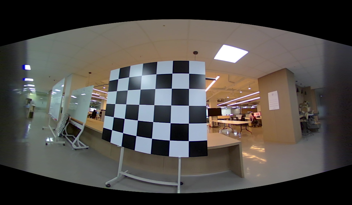
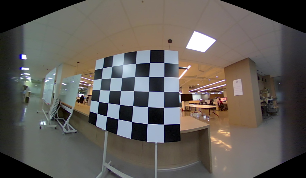
Resampling the bundled fisheye through each chart (every sample taken from the real DoubleSphereCamera.project) gives three genuine images:

Sphere (equirectangular)	Cylinder	Pinhole (gnomonic)

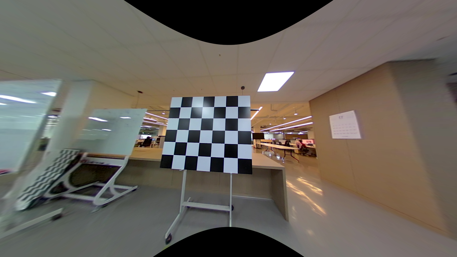widest; world verticals bow	verticals stay straight; height compressed	lines stay straight; periphery blows up, poles fall off the frame

And the morph — moving from one to another by blending the per-pixel ray and re-projecting, so the endpoints are the exact charts above (asserted to float precision in the render):

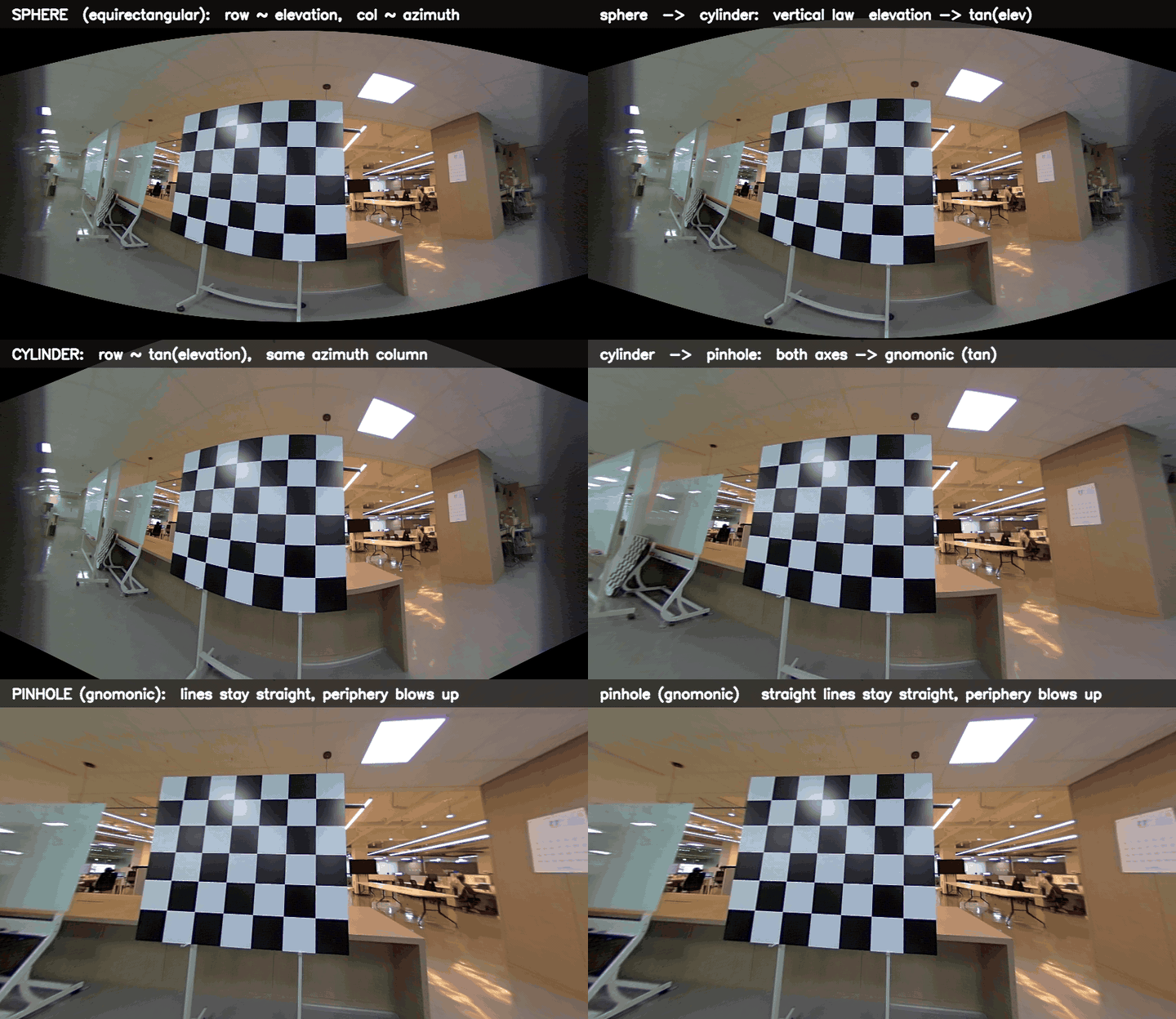
Watch the azimuth (horizontal) stay fixed from sphere to cylinder — only the rows slide as elevation re-spaces through $\tan$.

Then both axes bend through $\tan$ into the pinhole, and the top/bottom punch out to black: the

90° cone has nowhere to land on a flat plane (the Chapter 3 story, seen from the other side).

5. Proof on a real board: every corner survives every conversion¶

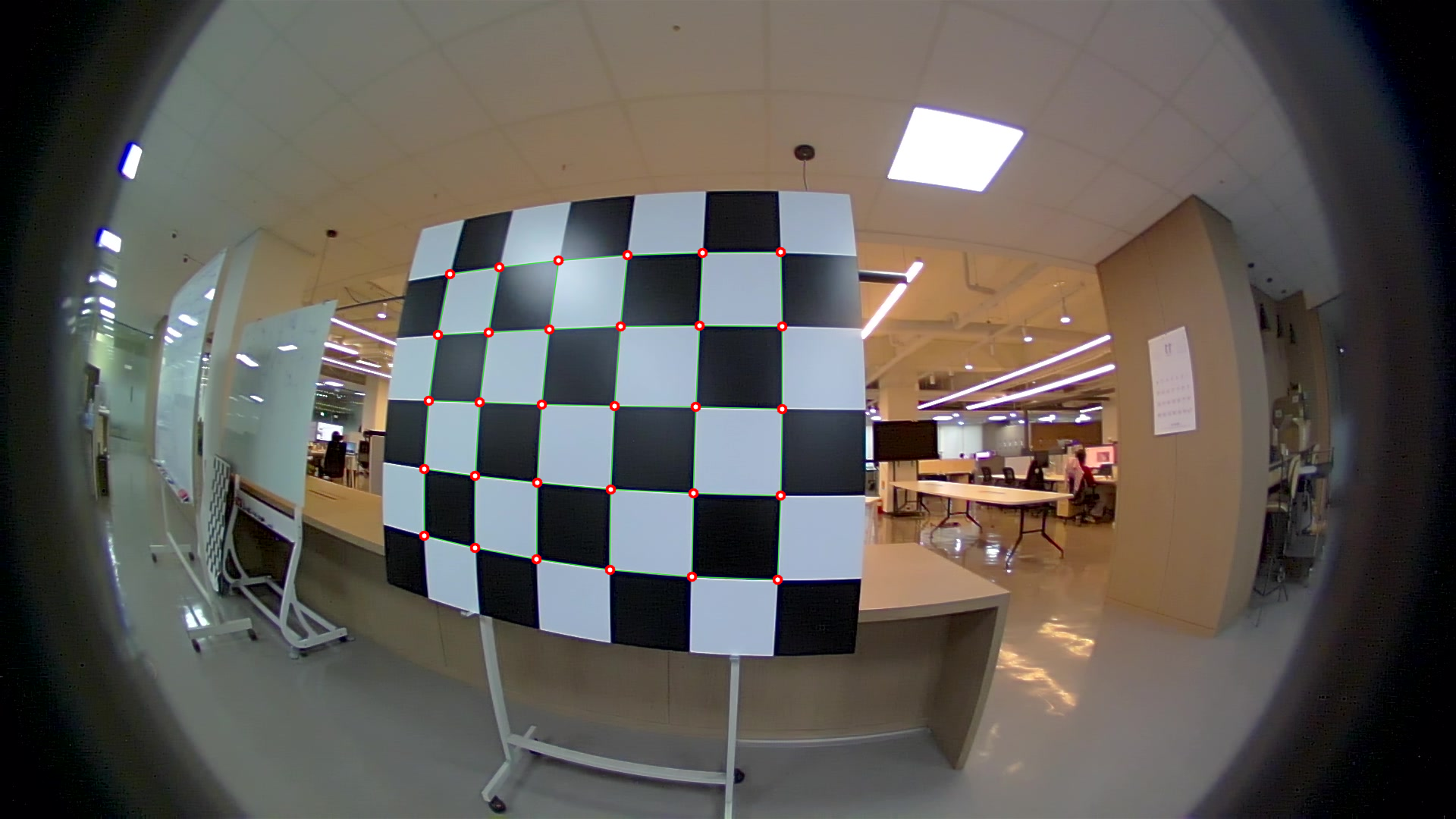
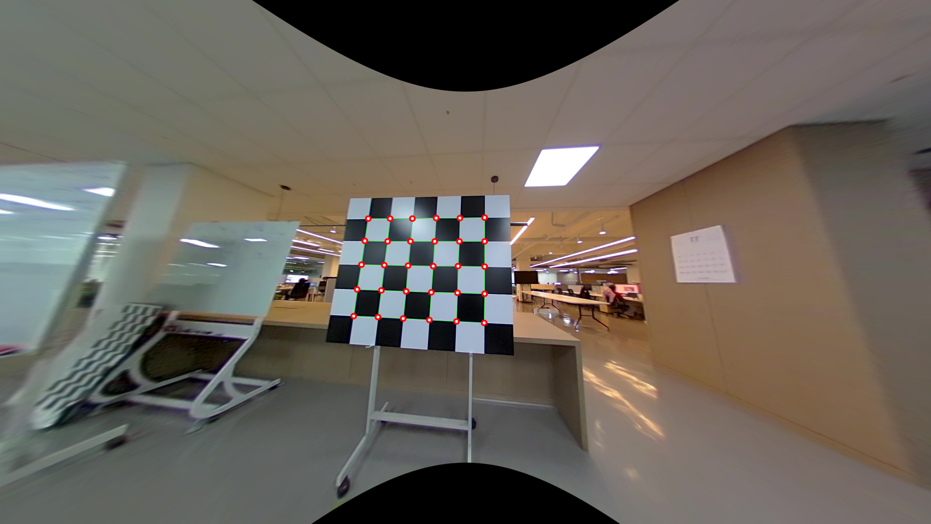
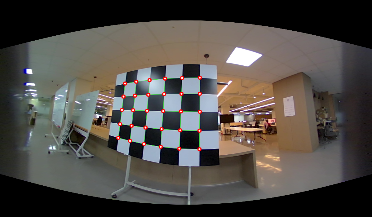
Pretty pictures aren't proof. The bundled fisheye has a checkerboard with 30 known corner pixels (anns.json) — a perfect ground-truth probe.

We push each raw corner through the conversion math, raw pixel → DS-unproject → ray → chart pixel, and draw it on each representation.

If the maps are right, every dot must land exactly on the checkerboard corner you can see in that image — even though the board is shaped completely differently in each chart.

The green grid connects the corners so you can watch the board bend while the dots stay put:

Raw fisheye	Pinhole (gnomonic)

Sphere (equirectangular)	Cylinder

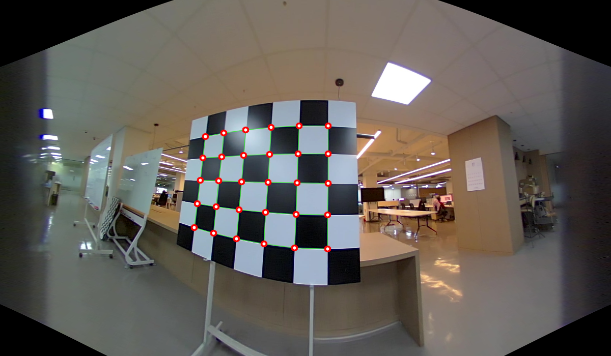The board bows in the sphere, straightens to a perfect rectilinear grid in the pinhole, and keeps its verticals straight in the cylinder — yet not one corner leaves its checkerboard intersection. That is the conversion math working, made visible.

The numbers behind the pictures¶

Round-trip every corner all the way back — raw → ray → chart pixel → ray → raw — and measure how far it lands from where it started (python examples/08_reproject_sphere_cylinder.py prints this table):

Representation	Mean round-trip error	Max	Corners checked
Sphere (equirectangular)	7.5e-14 px	2.3e-13 px	30 / 30
Cylinder	7.0e-14 px	2.3e-13 px	30 / 30
Pinhole (gnomonic)	7.4e-14 px	1.6e-13 px	30 / 30

1e-13 px is float64 round-off: a corner detected in the fisheye returns to within an atom's width of itself after a full trip through any representation.

The pictures and the table agree — the conversions move pixels between charts without losing a thing, which is exactly the property you need before trusting a representation for real 2D/3D work.

6. So — can you do 2D/3D tasks on these? Yes, with one caveat¶

Ray-based geometry transfers unchanged¶

Because every chart is just a relabelling of the same rays, anything ray-based is representation-agnostic and transfers directly:

Epipolar geometry still holds on bearing vectors:

\[\mathbf{x}_2^\top E\,\mathbf{x}_1 = 0\]

On the sphere image an epipolar line becomes an epipolar great circle.
Triangulation, PnP, bundle adjustment operate on rays, so they don't care whether you stored the measurement as a sphere, cylinder, or pinhole pixel. Spherical SfM and spherical stereo are standard for exactly this reason.
A landmark drawn "on the sphere" is literally its bearing vector — the honest geometric thing a fisheye measures.

The caveat is the cylinder. It is central only in azimuth; vertically it's a $\tan$ map that cannot represent the poles ($\pm 90°$ elevation sit at infinity). Running examples/08_reproject_sphere_cylinder.py prints the gap for one panorama height:

$ python examples/08_reproject_sphere_cylinder.py
Same image height, different elevation reach (top row of the panorama):
  sphere row 0   reaches elevation  62.7 deg
  cylinder row 0 reaches elevation  47.6 deg (tan compresses it; the poles sit at infinity)
---> 100%

A cylinder is fine for horizon-band work — panoramas, road scenes. The sphere has no such hole, though: it's the complete central model, which is the whole reason your Double Sphere camera carries a sphere inside it.

Don't triangulate near the caps

A cylinder silently drops the polar cone. Don't run full-sphere triangulation near its caps — the elevation gap measured above (47.6° vs. 62.7°) means points near the poles simply aren't representable in that chart.

One trap worth repeating

None of these charts give you intrinsics for free. The pretty equirectangular image is fisheye pixel → DS-unproject → ray → sphere pixel — the hard part (the genuine calibration that produced ξ, α, f, c) happens upstream, and the sphere just inherits it. A representation is only ever as correct as the calibration it was warped from.

Generated by a checked-in script: the morph's endpoint frames are asserted equal to the true single-model reprojections, so the animation can't drift from the library's geometry.

Chart	Column law (azimuth)	Row law (elevation)	Valid range
Sphere (equirectangular)	\(u = c_x + f\,\lambda\)	\(v = c_y - f\,\psi\)	full \(S^2\)
Cylinder	\(u = c_x + f\,\lambda\)	\(v = c_y - f\,\tan\psi\)	\(\lvert\psi\rvert<90°\)
Pinhole (gnomonic)	\(u = c_x + f_p\,\dfrac{x}{z}\)	\(v = c_y + f_p\,\dfrac{y}{z}\)	\(z>0\)