Projection validity and field of view — why a fisheye can't fully un-distort¶

Why does a rectified fisheye image always have a black border, and why are some pixels impossible to keep?

This page explains the geometry behind the Double Sphere model's field of view: the exact half-space test that decides which 3D rays are projectable, why that boundary sits past 90°, and why no single pinhole image can hold the result.

It is the "why" companion to the hands-on Chapter 3 tutorial; read this when you want the derivation and the proof, not the recipe.

Every claim below is checked against the implementation in ds_msp/models/ds_math.py (ds_project), so the math and the code can't drift.

The boundary is a tilted half-space, not `z > 0`¶

The Double Sphere projection \(\pi(\mathbf{x})\) is not defined for every 3D point. The naive guess for "can the camera see this point?" — is it in front of the camera? — is

\[z > 0.\]

For a fisheye that test is wrong. It is the single most common implementation bug: it silently discards every ray past 90°, capping a lens designed for more than 180° at exactly 180°.

The exact projectability condition (Usenko et al. 2018, Eq. 43–45) is a tilted half-space:

\[z > -w_2\, d_1, \qquad d_1 = \sqrt{x^2 + y^2 + z^2}\]

The tilt coefficient \(w_2\) is a constant built from the model's distortion parameters \(\alpha\) and \(\xi\) through an intermediate term \(w_1\):

\[ w_1 = \begin{cases} \dfrac{\alpha}{1-\alpha} & \text{if } \alpha \le 0.5 \\[2ex] \dfrac{1-\alpha}{\alpha} & \text{if } \alpha > 0.5 \end{cases} \qquad w_2 = \frac{w_1 + \xi}{\sqrt{2\, w_1 \xi + \xi^2 + 1}} \]

This is exactly what ds_project computes: the piecewise \(w_1\), then \(w_2\), then the mask valid = (z > -w2 * d1) & (den > 1e-8).

The second clause only guards the projection denominator against a near-zero divide. The geometry lives entirely in the tilted half-space \(z > -w_2 d_1\).

The crucial consequence follows from the sign of the tilt. Because

\[w_2 > 0,\]

the test admits points with \(z \le 0\) — rays that point slightly behind the camera's own side. That is precisely why the model represents a field of view greater than 180°.

A \(z > 0\) test would reject those rays and quietly cap the FOV at a hemisphere.

This library does not make that mistake; the comment in ds_project says so explicitly.

Reading the half-space as a maximum incidence angle¶

The half-space is easier to picture as an angle. Take a unit-length ray at incidence angle \(\theta\) from the optical axis:

\[d_1 = 1, \qquad z = \cos\theta.\]

Substituting into the test \(z > -w_2 d_1\) collapses it to a bound on the angle:

\[\cos\theta > -w_2 \quad\Longleftrightarrow\quad \theta < \theta_{\max},\]

\[\theta_{\max} = \arccos(-w_2).\]

Every ray out to \(\theta_{\max}\) is projectable; everything beyond it is outside the model's domain. This library was calibrated from a camera with

\[\xi = 0.183, \qquad \alpha = 0.809.\]

For it, the numbers are:

Quantity	Value
\(w_1\)	\(0.236\)
\(w_2\)	\(0.396\)
\(\theta_{\max} = \arccos(-w_2)\)	\(113.3°\)
Total accepted FOV (\(2\theta_{\max}\))	\(\approx 227°\)

So the camera accepts rays roughly 23° behind its own side — far past a 180° hemisphere.

The Chapter 3 tutorial cross-checks this formula at runtime against the full-precision calibration. It prints 113.4° from \(w_2 = 0.3967\) — a rounding-of-inputs difference from the 113.3° / 0.396 shown here.

A brute-force sweep confirms the closed form to the first decimal, so the formula is verified against the code, not just asserted.

The FOV zones, painted onto a real frame¶

The same valid region, mapped back onto a real fisheye image, splits the frame into three zones:

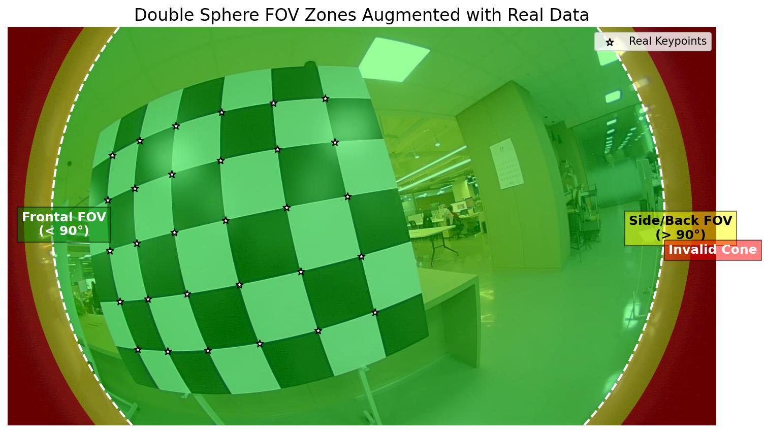
Green — frontal (\(\theta < 90°\)): ordinary forward rays. A pinhole camera could handle exactly these.
Yellow — side/back (\(90° \le \theta < \theta_{\max}\)): valid in Double Sphere (\(z \le 0\) here), but impossible to place in a single pinhole image. These are the rays the naive \(z > 0\) bug throws away.
Red (\(\theta \ge \theta_{\max}\)): outside the model's domain entirely — mathematically un-projectable.
White stars: real calibration keypoints, all sitting safely inside the valid region.

The picture to keep in mind: "in front of the camera" (the pinhole world) is a small green disc inside the much larger green-plus-yellow region a fisheye actually sees.

Why you can't undistort it all away¶

If the lens sees 227°, why does the rectified "pinhole view" always cut some of it off? Because a pinhole image plane is infinite at 90°. A ray at exactly 90° projects to

\[x / z \to \infty.\]

There is no finite image plane that holds the yellow zone. Those pixels are not lost to a bug — they are geometrically un-pinhole-able. The model is fine; the destination is the problem.

So rectification forces a trade between field of view and black border, controlled by a balance knob (see balanced_pinhole_K). The knob sets the rectified focal length as a fraction of the original:

balance = 0.0 gives the shortest focal: widest view, most of the scene kept.
balance = 1.0 gives the longest focal: narrowest view, least peripheral content.

A shorter focal packs more wide-angle scene into the frame, at the cost of corners that map to rays the source never captured — the black border.

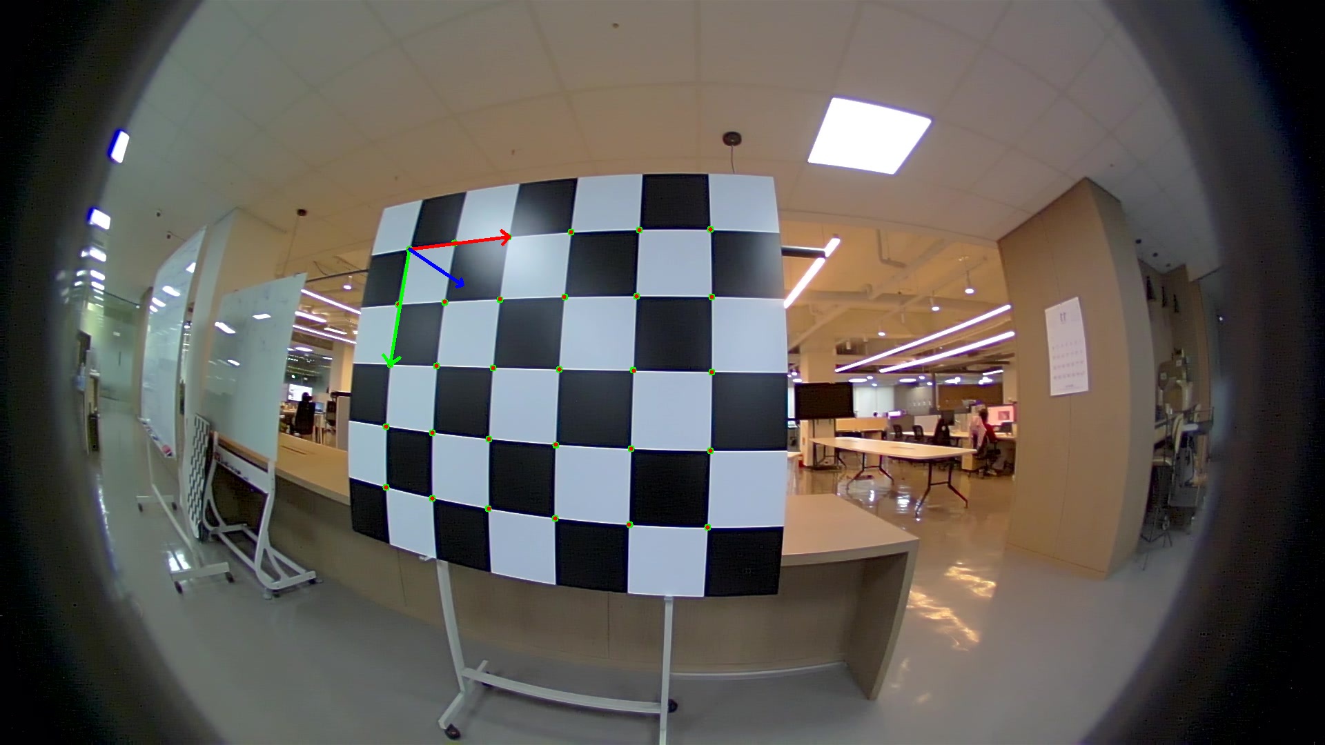
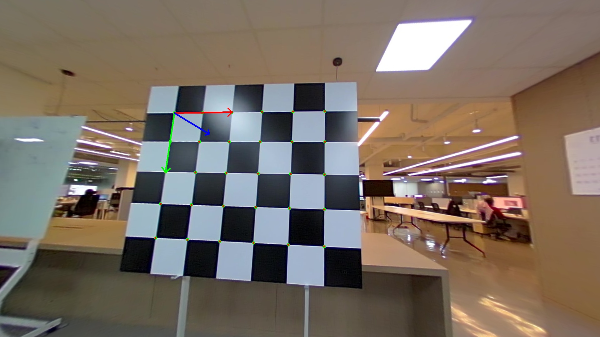
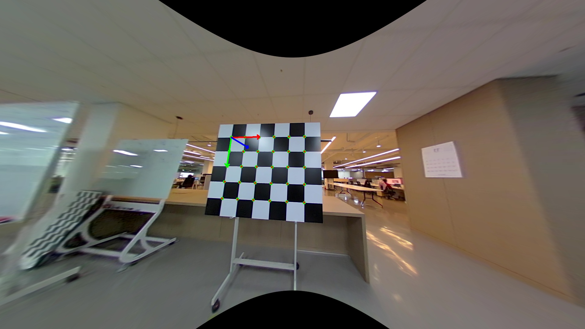
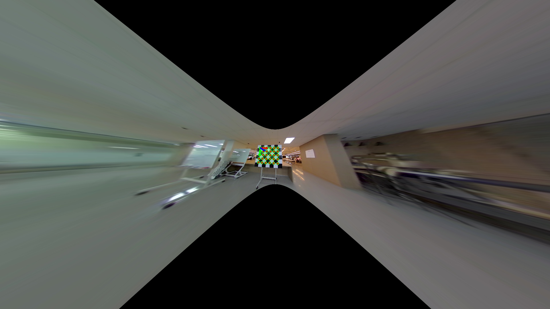
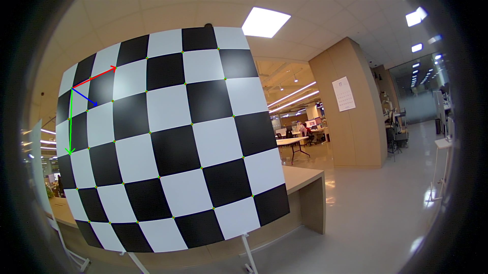
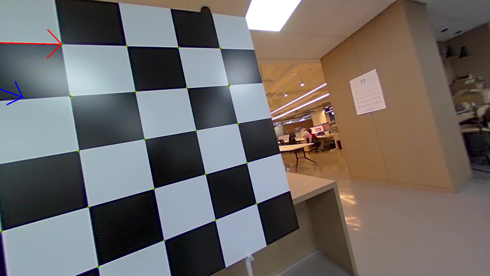
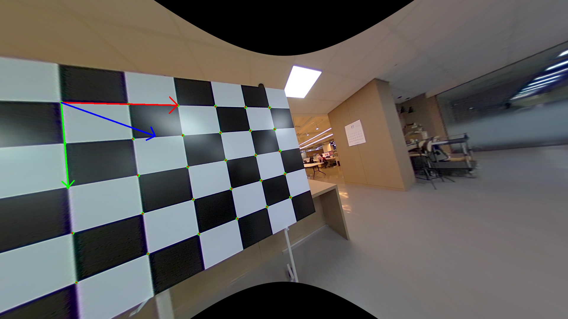
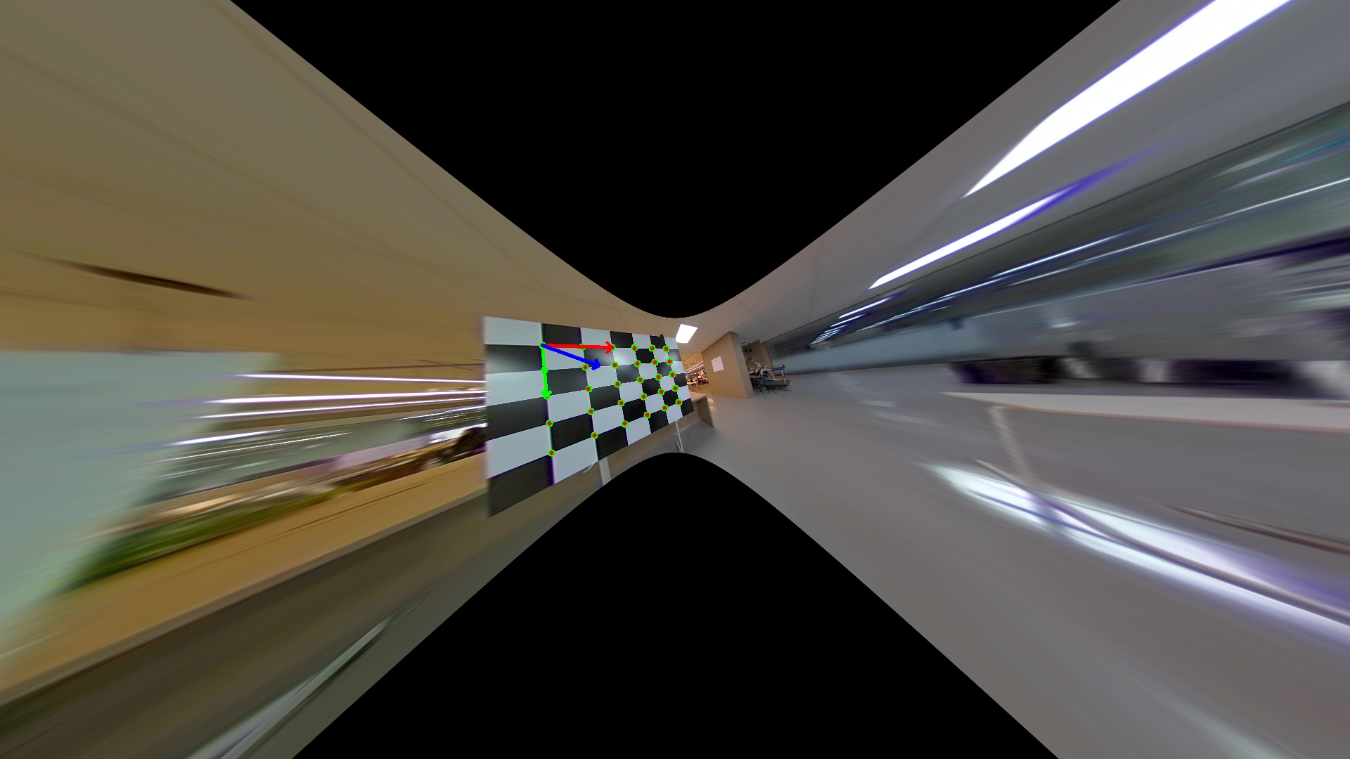
Verified on real data (assets/test_image.jpg, assets/test_image_96.jpg), the same distorted frame rectified three ways:

Distorted	Undistorted (crop)	Undistorted (whole)	Undistorted (zoom)

Crop (balance = 1.0) — the longest focal keeps only center-valid pixels: no black border, but the least field of view.
Whole (balance = 0.0) — the average of fx and fy, scaled to 0.4×, keeps every pixel that still maps to the plane: full content, with black borders at the corners.
Zoom (manually reduced focal) — uses a focal shorter than balanced_pinhole_K produces at balance = 0.0, so it is a hand-set focal rather than a balance value. The shorter focal captures even more wide-angle content and shrinks the center of the scene.

There is no setting that keeps the whole 227° in a flat image. You choose where on the trade-off curve to sit; you cannot leave it.

The equations below are exactly what ds_project and ds_unproject implement, shown in full for reference.

Forward / inverse equations

Forward projection. Start from the ray norm and the first-sphere shift:

\[d_1 = \sqrt{x^2 + y^2 + z^2}, \qquad z_1 = z + \xi d_1.\]

Then:

\[ d_2 = \sqrt{x^2 + y^2 + z_1^2}, \qquad \begin{bmatrix} u \\ v \end{bmatrix} = \begin{bmatrix} f_x\, x \big/ \big(\alpha d_2 + (1-\alpha) z_1\big) + c_x \\[1ex] f_y\, y \big/ \big(\alpha d_2 + (1-\alpha) z_1\big) + c_y \end{bmatrix} \]

This is the den = alpha * d2 + (1.0 - alpha) * z1 line in ds_project.

Inverse (unprojection) is closed-form. Start from the normalized image coordinates:

\[m_x = (u - c_x)/f_x, \qquad m_y = (v - c_y)/f_y, \qquad r^2 = m_x^2 + m_y^2.\]

The back-projection's validity depends on \(\alpha\):

for \(\alpha \le 0.5\), it is valid for all \(r^2\);
for \(\alpha > 0.5\), it is valid when \(r^2 \le 1/(2\alpha - 1)\).

The implementation's check in ds_unproject,

\[s = 1 - (2\alpha - 1)\, r^2 \ge 0,\]

is exactly this domain test.

Valid parameter domain:

\[\alpha \in [0, 1], \qquad \xi \in [-1, 1].\]

Outside it the model becomes non-injective: projection folds back on itself, so unprojection can no longer invert it.

What this lets you reason about¶

A fisheye's "can I see it?" test is a tilted half-space \(z > -w_2 d_1\), not \(z > 0\) — and the tilt is what buys the extra-hemispheric field of view.
That half-space is equivalently a maximum incidence angle \(\theta_{\max} = \arccos(-w_2)\); here \(\approx 227°\) of total FOV.
Undistortion to a pinhole cannot keep the part past 90°, so balance trades field of view against black border — a curve you position yourself on, not a defect.

Next: work through the runnable version in Chapter 3 — Projection validity & the >180° cone, or step back to Chapter 1 — Fisheye and camera models for where the Double Sphere model sits among the alternatives.