Chapter 2 — The Double Sphere model, from first principles¶
Run alongside this:
python examples/02_double_sphere_tumvi.py(after the setup). Read this, then read the printed numbers.
In Chapter 1 a camera model was a black box: a
project/unproject pair that happened to be inverses. This chapter opens one specific
box — Double Sphere (Usenko, Demmel & Cremers, 3DV 2018).
Its math is short, geometric, and exactly invertible. By the end you'll read
ds_math.py and
recognize every line.
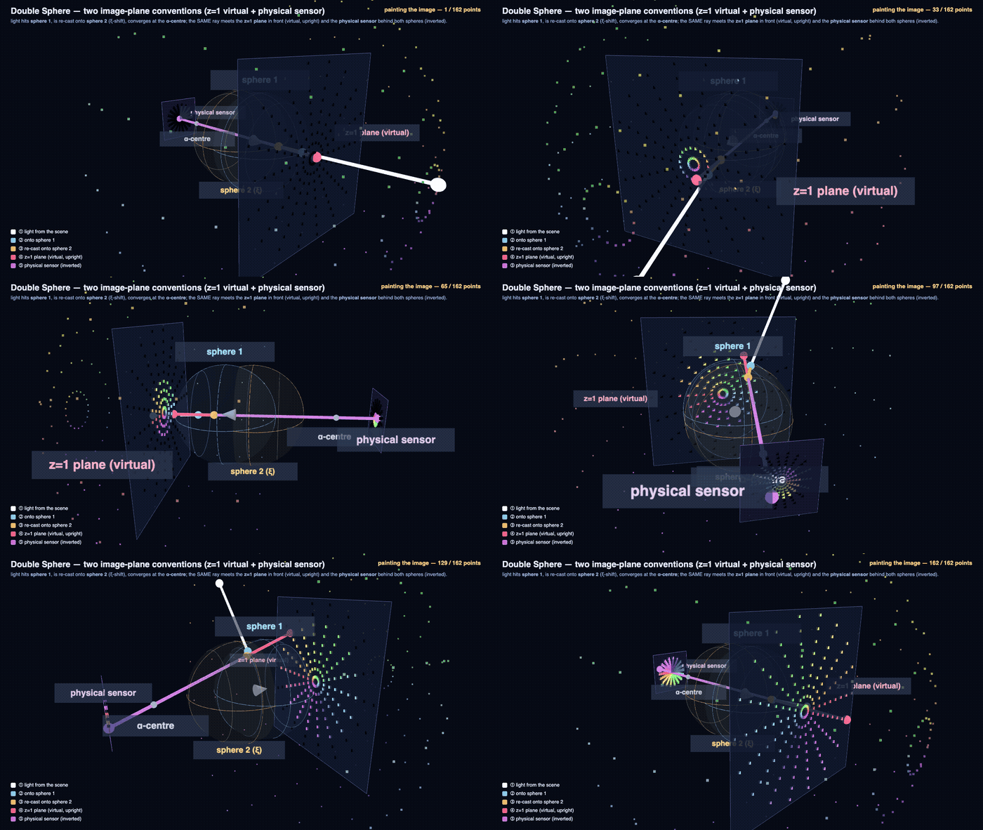
Follow the bright point as it travels 3D point → sphere 1 → sphere 2 → α-centre, while a colourful world of directions fills in the image.
The same projection ray meets two equivalent image planes — the model's normalized
z = 1 plane (virtual, upright) and the physical sensor behind both spheres (real,
inverted). Every coloured pixel is the exact ds_project of its 3D direction — even the ones
past 90°, which a normal camera cannot capture.
The model is radially symmetric, so a 2-D cross-section is the complete picture — the same construction with both image planes labelled:
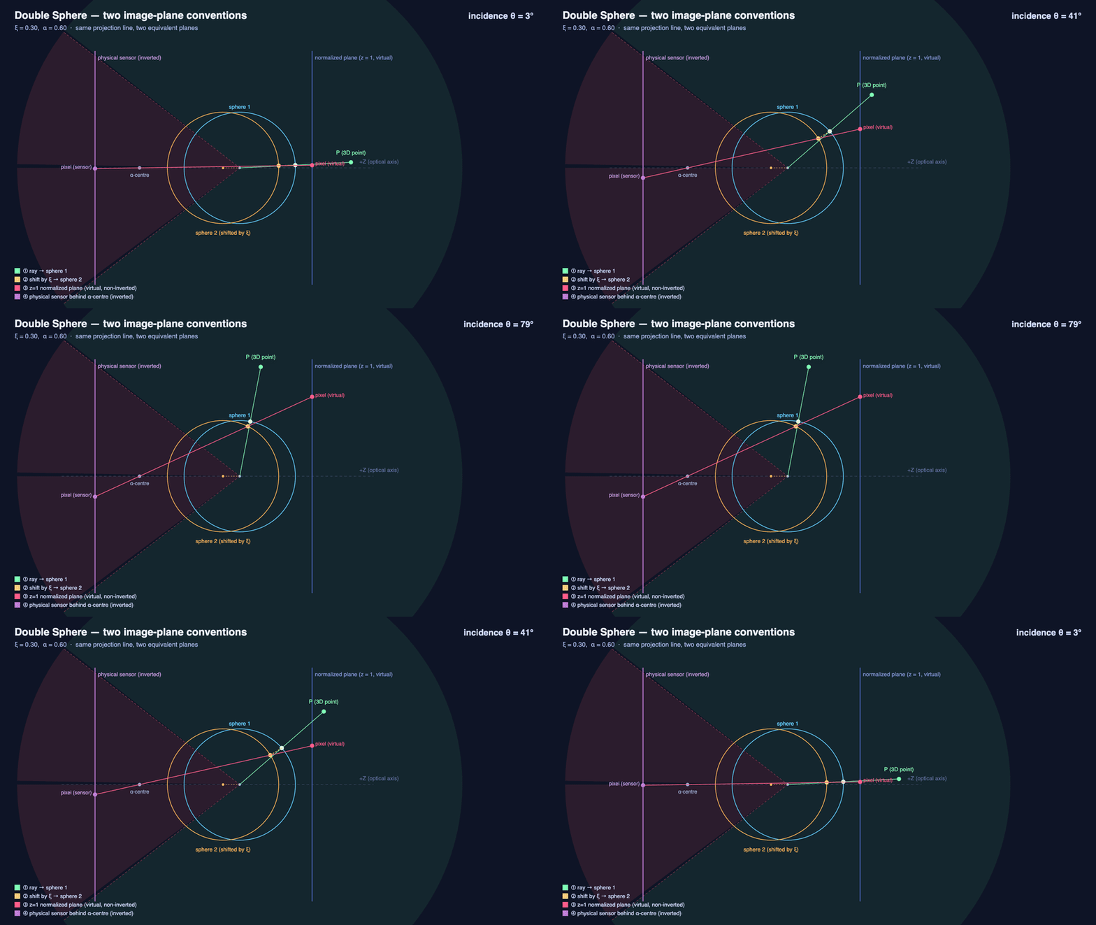
The two spheres sit between the 3-D world (right) and the sensor (left, behind the α-centre), matching the paper's figure; the z = 1 plane in front carries the equivalent upright image.
The sections below dissect each step.
You'll learn
- Derive Double Sphere's projection as two sequential unit-sphere projections — shifted by
ξ and blended by α — and read it directly in
ds_math.py.
- Why Double Sphere unprojects in closed form (one square root, no iteration), unlike
Kannala-Brandt's polynomial, which needs Newton's method.
- Verify projection and its closed-form inverse are exact to machine precision
(round-trip mean 2.17e-14 px, max 1.17e-13 px over 1600 real pixels).
- Use convert() to re-express TUM-VI's published
Kannala-Brandt calibration as Double Sphere, matching it to 0.025 px max reprojection
error over 179.8° of field of view.
Prerequisites
- Finish Chapter 1 — this chapter assumes project/
unproject and the CameraModel contract are already familiar.
- Same setup as Chapter 1; no new installs.
1. Why another model after Kannala-Brandt?¶
Kannala-Brandt (Chapter 1's model) describes the lens by a polynomial in the incidence
angle θ: r(θ) = θ + k1·θ³ + k2·θ⁵ + …. It fits well, but it has a practical wart:
unprojection has no closed form.
To go from a pixel back to a ray you must invert that polynomial numerically (Newton iterations) for every pixel, every frame.
In a VO/SLAM front-end unprojecting thousands of features per image, that adds up.
Double Sphere was designed to fix exactly this: it matches fisheye lenses as well as KB while keeping both projection and unprojection in closed form — no iteration, no root-finding.
That single property is why it shows up in modern visual-inertial systems (it's the model behind Basalt). The whole point of this chapter is to see why it inverts cleanly.
2. The geometric picture: two spheres¶
Pinhole projection divides by Z. That explodes as a ray approaches 90° (Z → 0).
The fix every wide-FOV model uses is the same idea: first map the ray onto a unit sphere (where nothing explodes), then do a perspective division from a shifted center.
Models differ only in where that second center sits.
Double Sphere uses two unit spheres in sequence, governed by two new numbers:
The three-step construction¶
- Project the 3D point onto a first unit sphere — just normalize it. Now every direction, even one 100° off-axis, is a finite point on a sphere.
- Shift by
ξ(xi) and project onto a second unit sphere.ξis the gap between the two sphere centers. This second bending is what lets the model curve enough for real fisheye glass. - Pinhole-project from a center blended by
α(alpha).αslides the projection center between "the second sphere's center" (α=1) and "one sphere-radius behind it" (α=0). It controls how much perspective foreshortening remains.
So Double Sphere = pinhole + two shape knobs: ξ (sphere spacing) and α (which
center you project from). Everything else (fx, fy, cx, cy) is the ordinary intrinsic
matrix you already know.
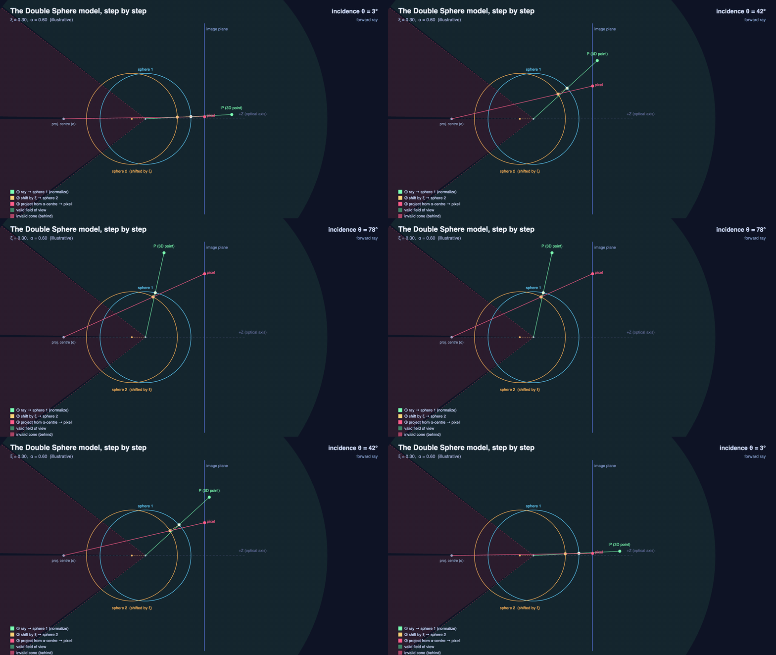
The construction in cross-section (the model is radially symmetric, so this slice is the
whole story): an incoming ray (green) lands on the first unit sphere, is shifted by
ξ onto the second sphere (orange), then projected from the α-blended centre
onto the image plane — a pixel (pink).
The shaded wedge is the valid field of view; watch θ climb past 90° and still land
inside it — the >180° reach a pinhole can never have.
(Rendered from the exact ds_project geometry — every point matches the library to ~1e-16.)
3. Read the projection in code¶
Here is the entire forward map from
ds_math.py — six lines of real
arithmetic, run below on a real detected corner (test_config.json) pushed out to an
arbitrary depth along its own ray:
"""Chapter 2 -- the Double Sphere forward map (Usenko et al. 2018).

These are the six lines of `ds_project` in `ds_msp/models/ds_math.py`, reproduced here
against the bundled real calibration and cross-checked against the real function -- so
the walkthrough can never silently drift from the library. The 3D point comes from
unprojecting a real detected corner (`test_config.json`) and pushing it out along its
own ray, which shows the central-projection property: only *direction* matters, so any
depth along that ray lands on the same pixel.
"""
import json

import numpy as np

from ds_msp.models.ds_math import ds_project, ds_unproject


def main() -> None:
    intr = json.load(open("test_config.json"))["intrinsics"]  # the bundled real calibration
    fx, fy, cx, cy = intr["fx"], intr["fy"], intr["cx"], intr["cy"]
    xi, alpha = intr["xi"], intr["alpha"]

    # A real detected corner, pushed out to 2.3 m along its own ray -- not unit length,
    # so d1 below is not trivially 1.
    u0, v0 = json.load(open("test_config.json"))["test_images"][0]["keypoints_2d"][0]
    ray, _ = ds_unproject(np.array([u0, v0]), fx, fy, cx, cy, xi, alpha)
    x, y, z = ray * 2.3
    print(f"3D point (camera frame, metres): x={x:.4f} y={y:.4f} z={z:.4f}")

    d1  = np.sqrt(x*x + y*y + z*z)          # distance to sphere 1  (normalize the ray)
    z1  = z + xi * d1                        # shift the z by xi  -> center of sphere 2
    d2  = np.sqrt(x*x + y*y + z1*z1)         # distance to sphere 2
    den = alpha * d2 + (1.0 - alpha) * z1    # the alpha-blended projection denominator
    u   = fx * x / den + cx
    v   = fy * y / den + cy

    print(f"d1={d1:.4f}  z1={z1:.4f}  d2={d2:.4f}  den={den:.4f}")
    print(f"u={u:.4f}  v={v:.4f}  (matches the original detected corner {u0}, {v0})")

    # cross-check against the real ds_project -- these six lines must never drift from it
    u_ref, v_ref, valid = ds_project(np.array([x, y, z]), fx, fy, cx, cy, xi, alpha)
    print(f"ds_project() agrees:  u={u_ref:.4f}  v={v_ref:.4f}  valid={bool(valid)}")


if __name__ == "__main__":
    main()
Match the code to the geometry¶
d1normalizes onto sphere 1.z1 = z + ξ·d1is the ξ shift — it pushes the point'sztoward the second sphere's center. Withξ = 0this line vanishes and the two spheres collapse into one (Double Sphere degenerates to the Unified Camera Model, UCM).den = α·d2 + (1−α)·z1is the α blend of the two possible denominators. Withα = 0you divide byz1(pure UCM-style); withα = 1you divide byd2. Real fisheyes land in between — TUM-VI's isα ≈ 0.71(the example prints it).- The last two lines are the pinhole division you've seen a hundred times, just with
denin place ofZ.
That's the whole model — two extra scalars on top of a pinhole.
The point above lands on the same pixel whether it sits 1 m or 100 m along that ray: only direction matters, the hallmark of a central camera.
4. Why it inverts in closed form¶
The reason Double Sphere unprojects without iteration: the forward map is a composition of a normalization and a quadratic perspective step. A quadratic can be solved with a square root rather than Newton's method.
You can see the solved result directly in
ds_unproject, walked below
for the same real corner and then cross-checked as a full round trip over all 30 bundled
corners:
"""Chapter 2 -- Double Sphere's closed-form unprojection (Usenko et al. 2018).

`mz` below is the solved quadratic from `ds_unproject` in `ds_msp/models/ds_math.py` --
one `np.sqrt`, no Newton iteration. Walked explicitly for one real detected corner, then
cross-checked as a full project(unproject(u)) round trip over all 30 bundled corners
(`test_config.json`) to show the closed form is the *exact* analytic inverse, not an
approximation.
"""
import json

import numpy as np

from ds_msp.models.ds_math import ds_project, ds_unproject


def main() -> None:
    intr = json.load(open("test_config.json"))["intrinsics"]  # the bundled real calibration
    fx, fy, cx, cy = intr["fx"], intr["fy"], intr["cx"], intr["cy"]
    xi, alpha = intr["xi"], intr["alpha"]
    pixels = np.array(json.load(open("test_config.json"))["test_images"][0]["keypoints_2d"])

    # walk the closed form for the first detected corner
    u, v = pixels[0]
    mx = (u - cx) / fx
    my = (v - cy) / fy
    r2 = mx*mx + my*my
    s = 1.0 - (2.0 * alpha - 1.0) * r2
    mz = (1.0 - alpha*alpha * r2) / (alpha * np.sqrt(s) + (1.0 - alpha))   # the closed form
    print(f"mx={mx:.4f}  my={my:.4f}  r2={r2:.4f}  mz={mz:.4f}")

    # full round trip over every real detected corner: project(unproject(u)) should
    # return u to float64 machine precision -- the closed form is an exact inverse.
    rays, valid_u = ds_unproject(pixels, fx, fy, cx, cy, xi, alpha)
    back_u, back_v, valid_p = ds_project(rays, fx, fy, cx, cy, xi, alpha)
    back = np.stack([back_u, back_v], axis=-1)
    good = valid_u & valid_p
    err = np.linalg.norm(back[good] - pixels[good], axis=1)
    print(f"pixels tested: {int(good.sum())} / {len(pixels)}")
    print(f"project(unproject(u)) round-trip: mean={err.mean():.2e}px  max={err.max():.2e}px")


if __name__ == "__main__":
    main()
No loop. That np.sqrt is the analytic inverse of the quadratic in §3. 1e-14 px is
float64's last bit — this isn't "close enough", it's the model is its own exact inverse.
Tip
The same precision holds at full scale. examples/02_double_sphere_tumvi.py runs the
identical round trip over 1600 real TUM-VI pixels:
Contrast Chapter 1's verify-don't-trust habit: this is proof, not a plausibility argument.
Note
The s ≥ 0 and sqrt_arg ≥ 0 checks in the code are where rays that the lens physically
can't see get flagged invalid — that's Chapter 3.
5. Is Double Sphere expressive enough for a real lens?¶
A model that inverts cleanly is useless if it can't actually fit real glass. TUM-VI's authors calibrated their fisheye and published it as a Kannala-Brandt model.
Can a Double Sphere model describe the same camera? The example re-expresses it with the
library's own convert() —
sample pixels, unproject through the reference, seed, then Levenberg-Marquardt refine with
the model's analytic Jacobian.
Measuring agreement across the frame¶
0.025 px maximum disagreement across a ~180° field — Double Sphere has the expressive power to capture this lens to a fortieth of a pixel.
Note
Why does fx change from 191 to 240? Focal length is model-relative — the same lens has a
different fx under KB vs DS because the denominators differ. The true paraxial (near-axis)
focal is fx_DS/(1+ξ). A whole deep-dive proves this:
are two models the same camera?. What's
invariant is where rays land, not the raw numbers.
Tip
This is model conversion, not calibration. We re-expressed one set of published numbers as another model's numbers — no images, no board, no detected corners.
Proving the model on real measurements is the capstone: detect AprilGrid corners in TUM-VI's raw calibration footage and bundle-adjust intrinsics from scratch that land on the published reference. Do Chapter 2, then jump to it — it's the artifact everything here builds toward.
Try it yourself¶
- In the example, after
convert(), printds.xiwhile forcingxi = 0(DoubleSphereModel(ds.fx, ds.fy, ds.cx, ds.cy, 0.0, ds.alpha)) and re-measure the reprojection error. How much worse does the single-sphere (UCM) fit get? That gap is what the second sphere buys you. - Convert to
EUCMModelandUCMModelinstead and compare their max reprojection error to Double Sphere's. Which models reproduce this lens best? - Run the round-trip grid (§4) out to the image corners (
np.linspace(0, W, …)) and watch how many pixels drop out of the valid mask near the edge — a preview of Chapter 3.
Next: the capstone — calibrate this camera for real from AprilGrid footage and match the published numbers.
Or continue the theory thread with Chapter 3 — projection
validity and the >180° cone (why z > 0 is the classic fisheye bug).