Chapter 1 — Fisheye lenses & what a "camera model" actually is¶

Run alongside this: python examples/01_realdata_fisheye_tumvi.py (after the setup). Read this, then read the printed numbers.

You'll learn - Why a pinhole model breaks for fisheye lenses (X/Z blows up past 90°), and what a "camera model" actually is: a project/unproject pair sharing one CameraModel contract. - How to load a real published calibration — TUM-VI's Kannala-Brandt intrinsics, straight from their Kalibr YAML — instead of calibrating one from scratch. - How to verify project and unproject are true inverses on real pixels, to machine precision (mean round-trip 1.55e-14 px, max 9.10e-14 px over a 1600-pixel grid). - How fisheye undistortion works, and why the balance knob trades field of view against black border in the rectified output.

Prerequisites - None — this is the first chapter. - Install the core library and the TUM-VI dataset:

uv pip install -e .
bash scripts/download_datasets.sh tumvi

(see the project setup for details).

1. The problem with straight lines¶

A pinhole camera has one defining property: straight lines in the world stay straight in the image. It's the model behind cv2.solvePnP, most SfM, and the matrix K you've seen a hundred times.

It works because projection is a clean perspective division: u = fx·X/Z + cx.

A fisheye lens deliberately breaks this to buy field of view — often > 180°, more than a hemisphere. Run the example and open results/learn/01_fisheye_raw.png: the ceiling lights bow into arcs. A pinhole model literally cannot describe this.

Note

Worse than "can't describe it": X/Z blows up as a ray approaches 90° off-axis (Z → 0), and goes nonsensical beyond it (Z < 0, i.e. light from behind the pinhole). You need a different model.

2. A camera model is a pair of functions¶

Strip away the mystique. A camera model is just two maps plus a handful of numbers (the intrinsics):

project: 3D point in the camera frame → 2D pixel. (X,Y,Z) ↦ (u,v)
unproject: 2D pixel → 3D unit ray (bearing). (u,v) ↦ (x,y,z), ‖·‖ = 1

That's the entire interface. In this library it's literally the CameraModel contract every model implements. Pinhole, Double Sphere, Kannala-Brandt, and the rest only differ in the math inside those two functions — same interface, swappable internals.

examples/01_realdata_fisheye_tumvi.py puts this to work on a real TUM-VI calibration (it needs the dataset from the setup, so this excerpt doesn't run standalone):

cam, (W, H) = load_kalibr_with_resolution(CAMCHAIN, cam="cam0")
rays, ok = cam.unproject(pix)   # 2D pixels -> 3D unit bearing rays
back, ok2 = cam.project(rays)   # 3D rays   -> 2D pixels again

3. A calibration is just numbers in a file¶

We don't calibrate anything in this chapter — we load a calibration that the TUM-VI dataset authors already computed and published, straight from their Kalibr YAML. Running the example prints the loaded model:

$ python examples/01_realdata_fisheye_tumvi.py
[1] loaded published TUM-VI cam0 calibration -> kb model (512x512)
    KannalaBrandtModel(fx=190.978, fy=190.973, cx=254.932, cy=256.897, k=[0.00348, 0.00072, -0.00205, 0.00020])

Six-plus numbers fully describe this fisheye camera:

fx, fy — focal lengths, in pixels.
cx, cy — the optical center.
k — four coefficients shaping the radial distortion.

TUM-VI's file says pinhole + equidistant, which is the Kannala-Brandt model — the same one behind OpenCV's cv2.fisheye.

The library reads it and hands you a working object. (Later chapters swap in the Double Sphere model, which handles >180° more gracefully.)

4. The non-negotiable habit: verify, don't trust¶

Here's the habit that separates 3D-vision work from "it looked fine on my test image": project and unproject must be inverses.

Unproject a pixel to a ray, project it back, and you must land on the original pixel. The example measures exactly this on a grid of 1600 real pixels:

$ python examples/01_realdata_fisheye_tumvi.py
[2] project(unproject(x)) round-trip on 1600 pixels: mean=1.55e-14px  max=9.10e-14px   (≈machine precision)

1e-14 is machine precision for float64 — the functions are inverse to the last bit the hardware can represent. If that number were 0.3px instead, your unprojection has a bug, full stop.

Always have a number that proves correctness. It's how you debug, and later, it's how you earn a reviewer's trust.

Note

Not every pixel is valid: some lie outside the lens's image circle, and not every 3D ray is projectable. A correct model tells you which — via the ok masks above. Chapter 3 is entirely about that validity boundary for >180° lenses.

5. Undistortion: "what would a pinhole have seen?"¶

Finally the example rectifies a real frame into a virtual pinhole view and saves results/learn/01_fisheye_rectified.png. Compare it to the raw frame: the bowed ceiling lines are now straight.

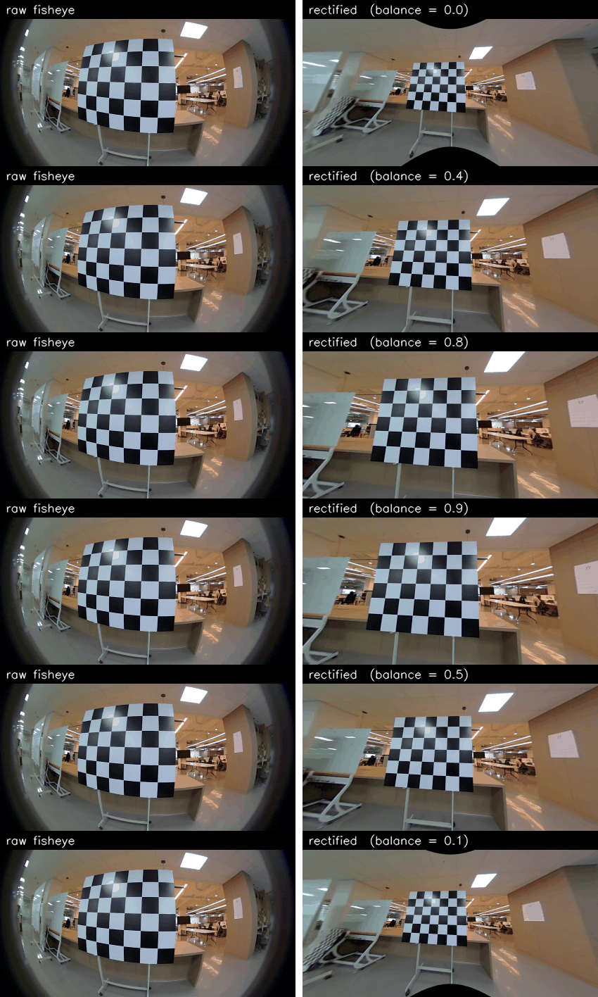
Left: the raw fisheye frame. Right: the rectified pinhole view as the balance knob sweeps from widest-FOV (more scene, black borders) to tightest-crop. The bent lines straighten out.

For every output pixel, Undistorter.maps() builds a pinhole ray from a fresh K_new, then projects it through the fisheye model to find where to sample the source image.

The balance knob trades field of view for how much black border you tolerate.

This is why undistortion can't keep a full >180° FOV: a pinhole image plane is infinite at 90°, so the periphery has nowhere to go.

Tip

Wide-FOV pixels aren't lost to a bug — they're geometrically un-pinhole-able. A rectified frame can never keep more than a hemisphere; Chapter 3 measures exactly how much is lost.

Try it yourself¶

Re-run with balance=1.0 in the script — predict whether the rectified image gets more or less black border before you look.
Load cam="cam1" (the other stereo camera) and confirm its intrinsics differ slightly.
Widen the verification grid toward the image edge (np.linspace(2, W-2, …)) and watch how many pixels fall outside the valid mask.

Next: Chapter 2 opens up the Double Sphere model, derives its projection from a two-sphere geometric picture, and uses it to reproduce TUM-VI's published calibration to a fortieth of a pixel.